In this tutorial you will learn how to run a basic simulation using HemeLB. This will look at aspects from planning a simulation, writing input files, launching the simulation and visualising the results.
Model layout
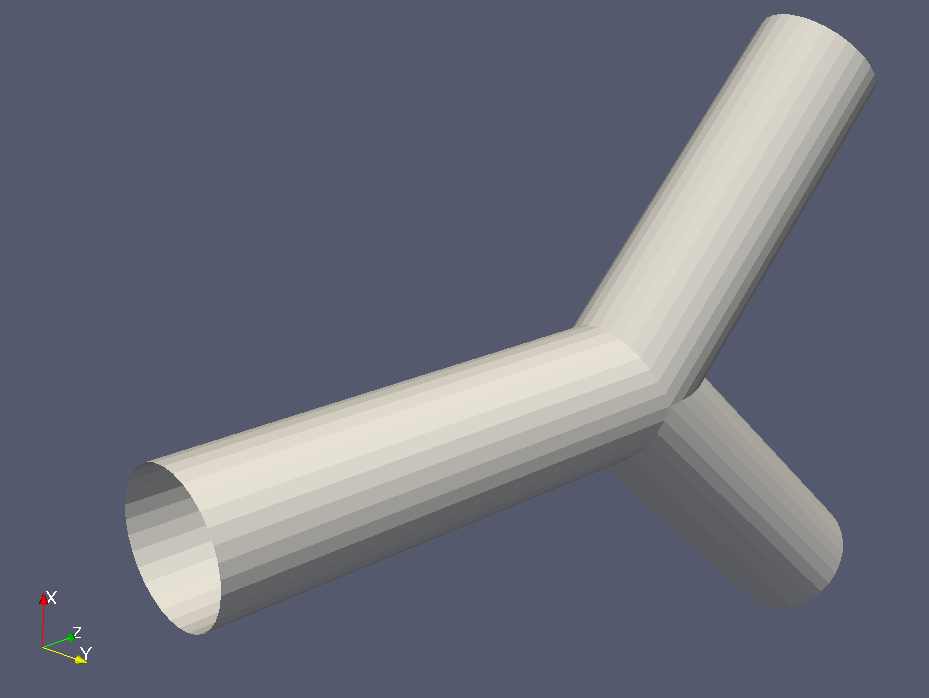
We will be running through an example of pressure driven flow through a bifurcation available in the HemeLB download. This model highlights a number of useful introductory options for running a simulation with HemeLB.
Background information
When planning a simulation using HemeLB (or any other code), many features need to be considered before running calculations:
- Wall behaviour
- Inlet and outlet conditions
- Fluid properties
- LBM parameters
- Resolution of domain in time and space
- Duration of simulation
- Output information
In HemeLB, the first two items are set in the compilation of the code with specific parameter values for inlets/outlets set in the input files. The LBM relaxation model is also set during the code compilation with the single-relaxation-time BGK model typically being used. HemeLB also assumes a fluid with the viscosity of blood is flowing in the domain. The BGK model links viscosity, lattice spacing, and simulation timestep to the relaxation parameter $\tau$ by,
$\nu = \frac{1}{3} \left( \tau - \frac{1}{2} \right) \frac{\Delta x ^2}{\Delta t}. $
Here:
- $\nu$ - Fluid viscosity
- $\Delta x$ - Lattice spacing
- $\Delta t$ - Time step
This relationship puts physical and practical limits on the values that can be selected for these parameters. In particular, $\tau > \frac{1}{2}$ must be imposed for a physical viscosity to exist. Generally, a value of $\tau \approx 1$ gives the most accurate results.
Next step: Input files
Move on to the next section to see how these are placed in the input file for a simulation.